Rendered map of New York City area showing detailed geographic features

Weekend Project: Building a High-Performance Maps Renderer in Rust

Weekend projects are supposed to be small, contained experiments. You pick a technology you want to try, spend Saturday afternoon tinkering, maybe Sunday morning polishing, and you've learned something new.

But sometimes you download a 2GB OpenStreetMap file of New York City, think "how hard could it be to render this?", and three weekends later you've built a parallel map rendering engine that processes millions of geographic features and generates stunning visualizations.

That's what happened here.

The "Something New Every Weekend" Challenge

Last summer, I committed to learning something completely new every weekend. Not just reading about it or watching tutorials, but actually building something. The rules were simple:

Pick a technology or concept I'd never touched
Build something functional by Sunday night
Share what I learned (the failures included)

This particular weekend, I was curious about two things: Rust's performance claims and how mapping software actually works. Google Maps makes it look effortless, but what does it take to turn raw geographic data into those beautiful visualizations we see every day?

Spoiler alert: it's way more interesting than I expected, and yes, I had to make sure it supported airports. Because planes. I like planes.

The Raw Material: OpenStreetMap Data

OpenStreetMap (OSM) is basically Wikipedia for geographic data. It's a massive, crowd-sourced database of roads, buildings, rivers, airports, and pretty much everything else you can see from above. The data comes in .pbf files (Protocol Buffer Format) that are compressed but still enormous.

The New York City metro area file? 2.1GB compressed. Uncompressed, we're talking about millions of geographic features:

Highways: Every road from interstates to tiny residential streets
Waterways: Rivers, streams, lakes, coastlines
Railways: Subway lines, freight tracks, abandoned rails
Buildings: Individual structures with precise outlines
Natural features: Parks, forests, beaches
Aeroways: Runways, taxiways, terminal buildings (my personal favorite)
Multipolygons: Complex shapes like airports or large parks

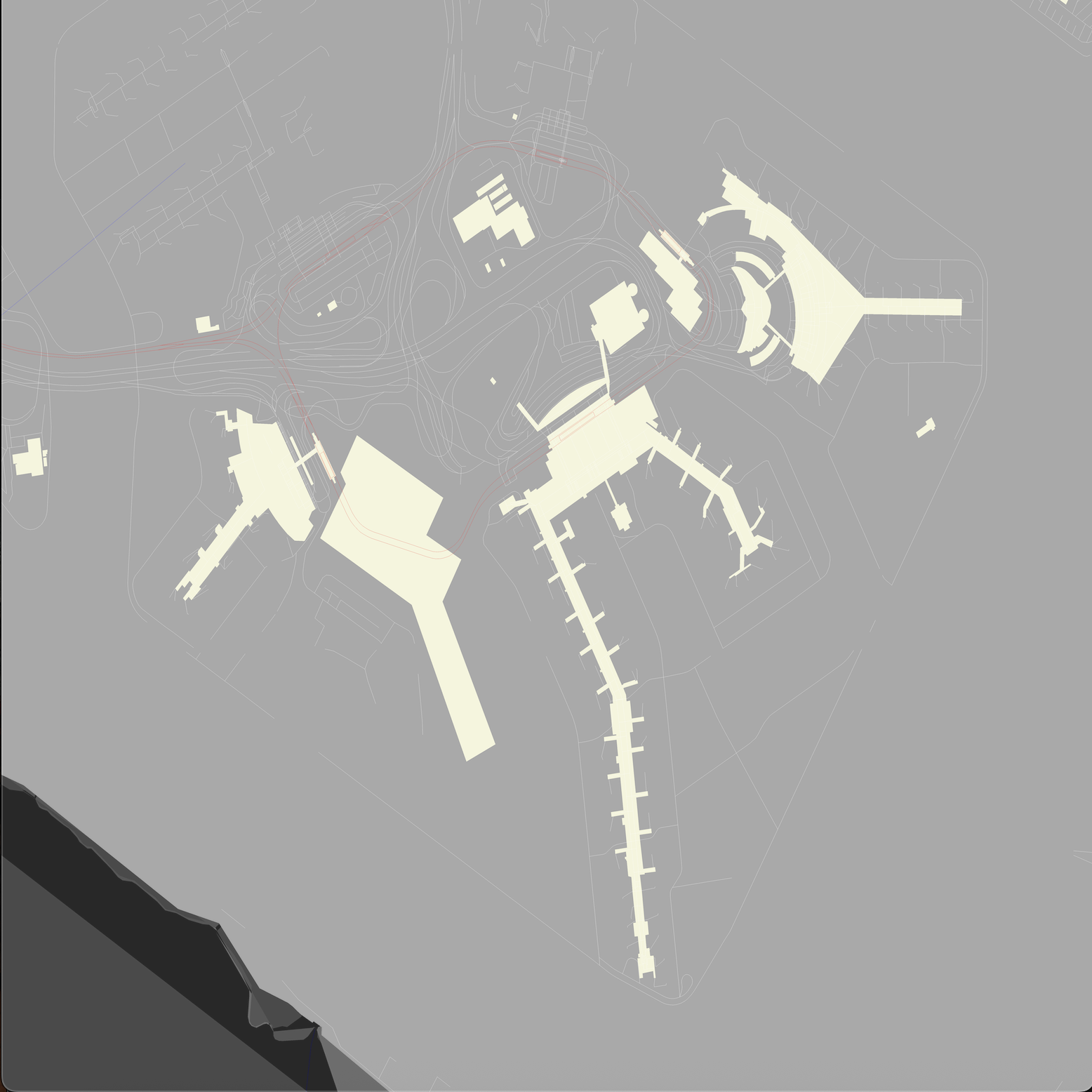
JFK Airport rendered with detailed runway and terminal layouts

JFK Airport showing runway layouts and terminal buildings in detail

Here's what makes this challenging: each feature is defined by a series of coordinate points (longitude, latitude), and a single "way" (OSM's term for a connected line or polygon) can have hundreds of points. The NYC dataset contains roughly 8 million nodes and 800,000 ways.

That's a lot of data to parse, process, and render efficiently.

Weekend #1: "How Hard Could Parsing Be?"

My first naive approach was simple: read the file, extract coordinates, draw lines. I figured I'd have a basic map by Saturday evening.

Three hours later, I was staring at Rust compiler errors and wondering why geographic data formats are so complicated.

Here's what I learned:

OSM Data Structure is Hierarchical

// Nodes: Individual points with coordinates
Node { id: 12345, lat: 40.7589, lon: -73.9851 }

// Ways: Collections of nodes forming lines or polygons
Way {
  id: 67890,
  nodes: [12345, 12346, 12347],
  tags: {"highway": "primary", "name": "Queens Boulevard"}
}

// Relations: Collections of ways forming complex shapes
Relation {
  id: 111213,
  members: [way_67890, way_67891],
  tags: {"type": "multipolygon", "aeroway": "aerodrome"}
}

You can't just read the file sequentially. You need to:

Parse all nodes first (to build a coordinate lookup table)
Process ways (connecting node IDs to actual coordinates)
Handle relations (which group ways into complex shapes like airports)

The osmpbfreader Crate Saves the Day

After wrestling with Protocol Buffer specs, I discovered the osmpbfreader crate. It handles all the binary parsing complexity:

use osmpbfreader::{OsmId, OsmObj, OsmPbfReader, Relation, Way};

pub fn read_osm_data(filename: &OsStr) -> (
    HashMap<i64, (f64, f64)>,  // Node coordinates
    Vec<WayCoords>,            // Highways
    Vec<WayCoords>,            // Waterways
    Vec<WayCoords>,            // Railways
    Vec<WayCoords>,            // Buildings
    Vec<WayCoords>,            // Natural features
    Vec<WayCoords>,            // Aeroways (!)
    Vec<Vec<WayCoords>>,       // Multipolygons
) {
    let r = std::fs::File::open(std::path::Path::new(filename)).unwrap();
    let mut pbf = OsmPbfReader::new(r);

    let mut nodes: HashMap<i64, (f64, f64)> = HashMap::new();
    let mut highways: Vec<WayCoords> = Vec::new();
    // ... other collections

    for obj in pbf.par_iter().map(Result::unwrap) {
        match obj {
            OsmObj::Node(node) => {
                nodes.insert(node.id.0, (node.lon(), node.lat()));
            }
            OsmObj::Way(way) => {
                let way_nodes = extract_way_nodes(&way, &nodes);
                match way.tags.get("aeroway") {
                    Some(_) => aeroways.push(way_nodes), // Airports!
                    None => {
                        if way.tags.get("highway").is_some() {
                            highways.push(way_nodes);
                        }
                        // ... handle other types
                    }
                }
            }
            // Handle relations for complex shapes
        }
    }
}

Notice that pbf.par_iter()? The crate supports parallel iteration out of the box. On my MacBook, this cut parsing time from 4 minutes to about 34 seconds.

By Sunday night of weekend #1, I had successfully parsed the NYC dataset and could categorize different feature types. No rendering yet, but hey, progress.

Weekend #2: "Rendering... How Hard Could It Be?"

Famous last words, right?

My initial rendering approach was embarrassingly simple: convert lat/lon coordinates to pixel coordinates, draw lines between consecutive points. I figured the image crate would handle everything else.

Four hours of debugging later, I learned why proper map rendering is an art form.

Challenge #1: Coordinate Conversion

Geographic coordinates (latitude, longitude) don't map linearly to screen pixels. The Earth is round, screens are flat, and projection matters.

For this project, I went with the simplest approach: treat the bounding box as a rectangle and scale linearly:

fn lon_lat_to_pixel(
    lon: f64, lat: f64,
    min_lon: f64, min_lat: f64,
    max_lon: f64, max_lat: f64,
    img_size: u32,
) -> (i32, i32) {
    let lon_range = max_lon - min_lon;
    let lat_range = max_lat - min_lat;

    let x = ((lon - min_lon) / lon_range * img_size as f64) as i32;
    let y = ((max_lat - lat) / lat_range * img_size as f64) as i32; // Note: flip Y

    (x, y)
}

This works surprisingly well for city-scale maps where distortion is minimal. For larger areas, you'd want proper projections like Web Mercator.

Challenge #2: Line Quality

My first rendered map had jagged lines, pixelated curves, and aliasing everywhere.

Wu's line algorithm is an anti-aliased line drawing technique that creates smooth, professional-looking lines:

fn draw_line_wu(img: &mut RgbaImage, x0: i32, y0: i32, x1: i32, y1: i32, color: Rgba<u8>) {
    let (dx, dy) = ((x1 - x0).abs(), (y1 - y0).abs());

    // Handle steep lines by swapping x/y coordinates
    let (mut x0, mut y0, mut x1, mut y1) = if dy > dx {
        (y0, x0, y1, x1)
    } else {
        (x0, y0, x1, y1)
    };

    if x0 > x1 {
        std::mem::swap(&mut x0, &mut x1);
        std::mem::swap(&mut y0, &mut y1);
    }

    let gradient = if x1 - x0 == 0 { 1.0 } else {
        (y1 - y0) as f32 / (x1 - x0) as f32
    };

    let mut intery = (y0 as f32) + gradient * 0.5;

    for x in x0..=x1 {
        // Draw two pixels with alpha blending for smooth lines
        plot(img, x, intery.floor() as i32, color, 1.0 - (intery - intery.floor()));
        plot(img, x, intery.floor() as i32 + 1, color, intery - intery.floor());
        intery += gradient;
    }
}

The alpha blending creates smooth lines. Instead of drawing hard-edged pixels, Wu's algorithm draws partially transparent pixels that create the illusion of smooth lines.

Challenge #3: Memory and Performance

Rendering the full NYC dataset at 4K resolution (4096x4096 pixels) was eating 16GB+ of RAM and taking 20+ minutes. That's not exactly weekend project friendly.

Time for some optimization.

Weekend #3: "Let's Make It Fast"

This is where Rust really shines. The language gives you fine-grained control over memory and concurrency without the usual pain of manual memory management.

Optimization #1: Tiled Rendering

Instead of creating one massive 24,576×24,576 pixel image, I switched to tiled rendering:

let tiles_x = 6;
let tiles_y = 6;
let img_size: u32 = 4096; // Each tile is 4K

let lon_step = (max_lon - min_lon) / tiles_x as f64;
let lat_step = (max_lat - min_lat) / tiles_y as f64;

let tiles: Vec<(usize, usize)> = (0..tiles_x)
    .flat_map(|x| (0..tiles_y).map(move |y| (x, y)))
    .collect();

tiles.par_iter().for_each(|&(x, y)| {
    let tile_min_lon = min_lon + x as f64 * lon_step;
    let tile_max_lon = tile_min_lon + lon_step;
    // Calculate tile bounds...

    let mut img: RgbaImage = RgbaImage::new(img_size, img_size);
    // Render only features that intersect this tile

    let file_name = format!("temp/{}_{}.png", x, y);
    img.save(&file_name).unwrap();
});

This approach has several benefits:

Memory efficient: Only one 4K image in memory per thread
Parallelizable: Each tile renders independently
Cacheable: Individual tiles can be cached and reused
Scalable: Want higher resolution? Just use more/larger tiles

Optimization #2: Rayon for Parallelization

Rust's rayon crate makes parallel processing almost trivial. That .par_iter() automatically distributes work across CPU cores:

use rayon::iter::{ParallelIterator, IntoParallelRefIterator};

// Parallel tile rendering
tiles.par_iter().for_each(|&(x, y)| {
    // Each tile renders on a separate thread
    render_tile(x, y, &highways, &waterways, /* ... */);
});

// Parallel image stitching
tile_coordinates.par_iter().for_each(|&(x, y)| {
    let tile_image = image::open(format!("temp/{}_{}.png", x, y)).unwrap();
    // Composite into final image
});

On my MacBook, this reduced total rendering time from 20+ minutes to about 3 minutes. Each tile renders in parallel, then they're stitched together into the final image.

Optimization #3: Smart Caching

Parsing that 2GB OSM file takes time, even with parallel processing. For iteration during development, I added a binary cache:

use serde::{Deserialize, Serialize};

pub fn load_cache<T: SerializableData>(filename: &str) -> Result<T, Box<dyn std::error::Error>> {
    let data = fs::read(filename)?;
    let cached_data: T = bincode::deserialize(&data)?;
    Ok(cached_data)
}

pub fn save_cache<T: SerializableData>(
    filename: &OsStr,
    data: &T
) -> Result<(), Box<dyn std::error::Error>> {
    let serialized_data = bincode::serialize(data)?;
    fs::write(filename, serialized_data)?;
    Ok(())
}

The first run parses the OSM file and saves the processed data. Subsequent runs load from cache in under 2 seconds instead of 12+ seconds. During development, this time savings adds up quickly.

The Rendering Pipeline: Layer by Layer

Modern maps aren't just lines on a white background. They're carefully composed layers that create depth and visual hierarchy. Here's my rendering order:

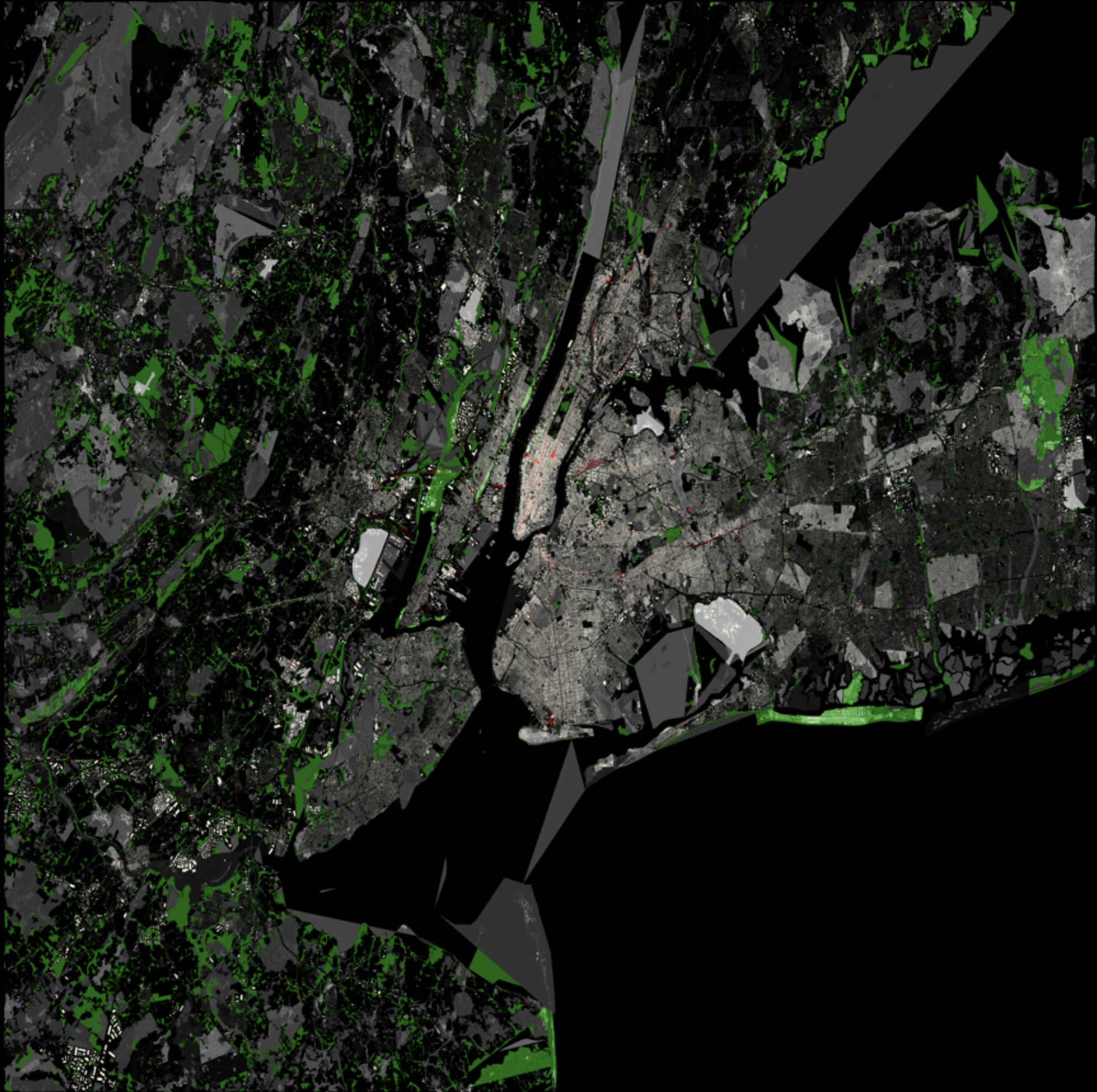
Complete architecture of the Rust maps renderer showing data flow, parallel processing, and layered rendering pipeline

Layer 1: Natural Areas (Green Foundation)

draw_buildings(
    &mut img, naturals,
    tile_min_lon, tile_min_lat, tile_max_lon, tile_max_lat, img_size,
    Rgba([0, 255, 0, 100]), // Semi-transparent green
);

Parks, forests, and other natural areas provide the base layer. I use semi-transparent green so other features can show through.

Layer 2: Multipolygons (Complex Shapes)

Airports, large parks, and other complex areas are often defined as multipolygons—collections of interconnected shapes:

fn draw_multipolygons(
    img: &mut RgbaImage,
    multipolygons: &[Vec<Vec<(f64, f64)>>],
    // ... parameters
    base_color: Rgba<u8>,
) {
    for multipolygon in multipolygons {
        for (i, polygon) in multipolygon.iter().enumerate() {
            // Slight color variation for each polygon part
            let color_adjustment = (i as u8 * 30) % 255;
            let adjusted_color = Rgba([
                (base_color[0] as u16 + color_adjustment as u16) as u8 % 255,
                base_color[1], base_color[2], base_color[3],
            ]);

            draw_polygon_mut(img, &polygon_points, adjusted_color);
        }
    }
}

Layer 3: Aeroways (Because Planes!)

This is where my aviation obsession shows. Airports get special treatment with detailed runway and taxiway rendering:

draw_buildings(
    &mut img, aeroways,
    tile_min_lon, tile_min_lat, tile_max_lon, tile_max_lat, img_size,
    Rgba([169, 169, 169, 255]), // Gray for runways/taxiways
);

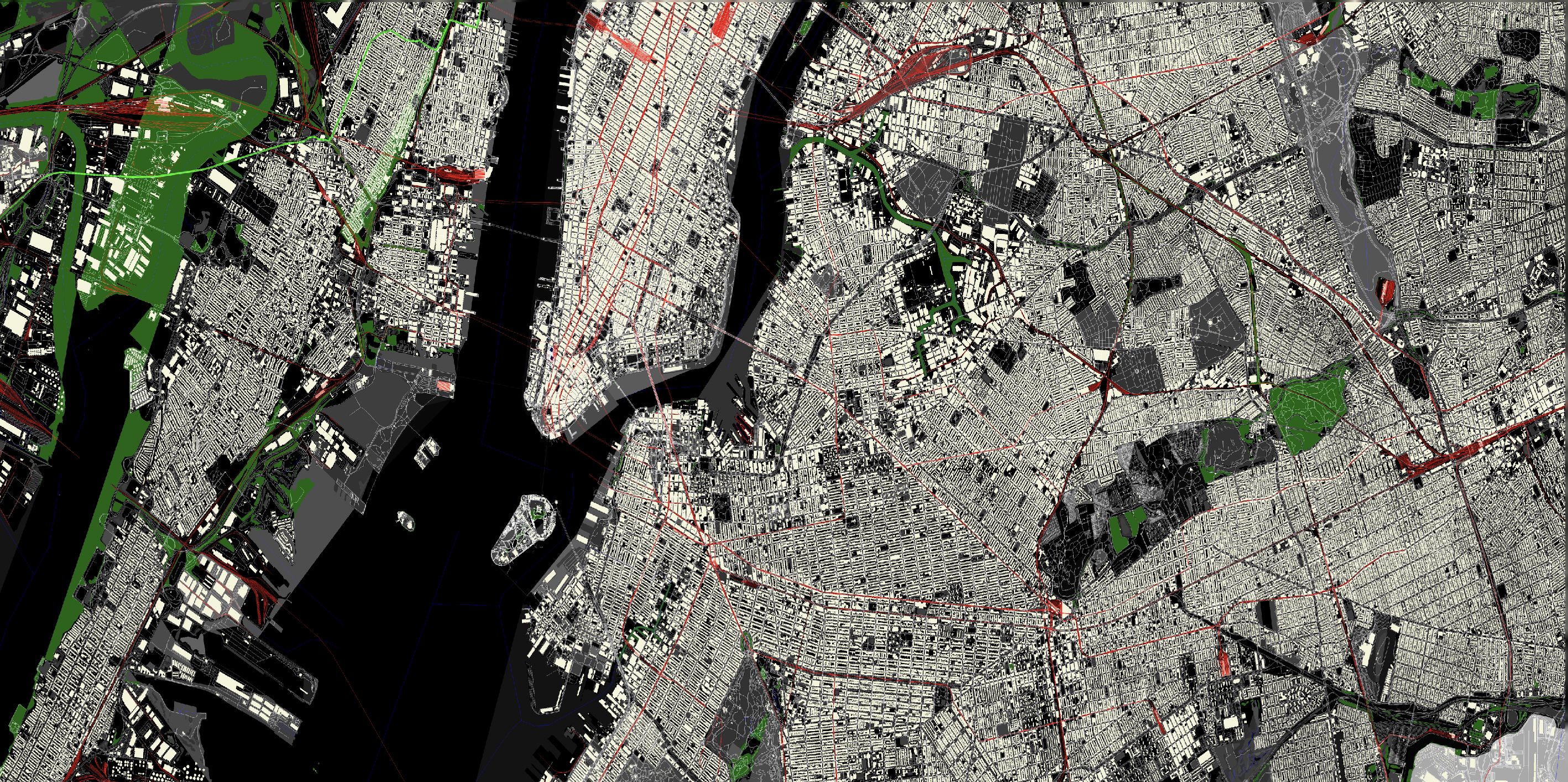
Full New York City map showing multiple airports and detailed infrastructure

NYC area showing Newark airports with detailed views of the city.

Layer 4-7: Buildings, Highways, Waterways, Railways

Each layer builds on the previous ones:

Buildings: Beige polygons for individual structures
Highways: White lines using Wu's algorithm for smooth rendering
Waterways: Blue lines for rivers and streams
Railways: Red lines for train tracks

The layering creates natural visual hierarchy. Water appears to flow under bridges, railways cross over roads, etc.

Bonus Feature: Pathfinding

Because I had some weekend time left, I added A* pathfinding capabilities. The idea is simple: click two points on the map and see the optimal route.

Building the Graph

pub fn build_graph(highways: &[Vec<(f64, f64)>]) -> HashMap<Coord, Vec<Edge>> {
    let mut graph = HashMap::new();

    for way in highways {
        for window in way.windows(2) {
            let (lon1, lat1) = window[0];
            let (lon2, lat2) = window[1];
            let start_id = Coord::new(lon1, lat1);
            let end_id = Coord::new(lon2, lat2);

            let cost = haversine_distance(lon1, lat1, lon2, lat2);

            // Bidirectional edges for roads
            graph.entry(start_id).or_insert_with(Vec::new)
                .push(Edge { target: end_id, cost });
            graph.entry(end_id).or_insert_with(Vec::new)
                .push(Edge { target: start_id, cost });
        }
    }
    graph
}

Haversine Distance for Accurate Costs

fn haversine_distance(lon1: f64, lat1: f64, lon2: f64, lat2: f64) -> i64 {
    let r = 6371e3; // Earth's radius in meters
    let phi1 = lat1.to_radians();
    let phi2 = lat2.to_radians();
    let delta_phi = (lat2 - lat1).to_radians();
    let delta_lambda = (lon2 - lon1).to_radians();

    let a = (delta_phi / 2.0).sin() * (delta_phi / 2.0).sin()
        + phi1.cos() * phi2.cos() * (delta_lambda / 2.0).sin() * (delta_lambda / 2.0).sin();
    let c = 2.0 * a.sqrt().atan2((1.0 - a).sqrt());

    ((r * c) * 1e8) as i64 // Scale for integer precision
}

The haversine formula calculates great-circle distances between points on Earth's surface. It's more accurate than simple Euclidean distance for geographic coordinates.

A* with the pathfinding Crate

use pathfinding::prelude::astar;

pub fn find_path(
    graph: &HashMap<Coord, Vec<Edge>>,
    start: Coord,
    goal: Coord,
) -> Option<(Vec<Coord>, i64)> {
    astar(
        &start,
        |&node| {
            graph.get(&node)
                .unwrap_or(&vec![])
                .iter()
                .map(|edge| (edge.target, edge.cost))
                .collect::<Vec<_>>()
        },
        |&node| haversine_distance(node.lon, node.lat, goal.lon, goal.lat), // Heuristic
        |&node| node == goal,
    )
}

The pathfinding crate handles the A* algorithm complexity. You just provide neighbor lookup, cost calculation, and heuristic functions.

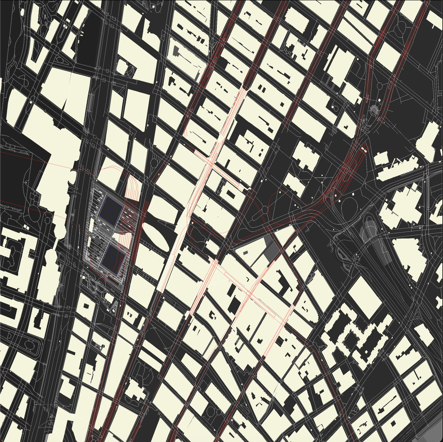
Close-up view of Manhattan streets with pathfinding visualization

Few blocks in Manhattan with roadways and railways rendered.

Performance: The Numbers

After three weekends of optimization, here's what the final system achieves:

Parsing Performance:

NYC OSM file (2.1GB): 12 seconds with parallel processing
Cache loading: 2 seconds for subsequent runs
Memory usage during parsing: ~4GB peak

Rendering Performance:

36 tiles (6×6 grid) at 4K each: 3 minutes total
Individual tile: 2-8 seconds depending on feature density
Memory usage: ~500MB per rendering thread
Final stitched image: 24,576×24,576 pixels (~2.3GB uncompressed)

Feature Processing:

8+ million nodes indexed
800,000+ ways categorized and rendered
Complex multipolygons (airports, parks) handled correctly
Pathfinding graph: 300,000+ navigable intersections

On my 8-core MacBook Pro, the system consistently processes the full NYC dataset in under 4 minutes from cold start (including parsing). With cached data, it's closer to 3 minutes.

What I Learned About Rust

This project was my deep dive into Rust, and it exceeded expectations in several areas:

Memory Safety Without Performance Cost

Rust's ownership system prevented several classes of bugs I would've hit in C++. No dangling pointers, no buffer overflows, no data races. But the performance was still excellent, comparable to optimized C code.

Fearless Concurrency

The rayon crate made parallel processing almost trivial. In other languages, I'd worry about thread safety, locks, and race conditions. Rust's type system makes data races impossible at compile time.

Cargo Ecosystem

The crate ecosystem is impressive. Complex tasks like:

OSM parsing (osmpbfreader)
Parallel iteration (rayon)
Image processing (image, imageproc)
Pathfinding algorithms (pathfinding)
Binary serialization (bincode, serde)

All handled by well-maintained, performant crates.

Error Handling

Rust's Result type forces you to handle errors explicitly. No silent failures, no mysterious crashes. Every function that can fail returns a Result, and you handle it or explicitly propagate it.

The Weekend Project Reflection

What started as "let me try Rust and see how map rendering works" turned into a fairly sophisticated system. But that's the beauty of weekend projects. They give you permission to explore deeper than you originally planned.

Key lessons:

Start simple: My first goal was just parsing the file. Each weekend built on the previous one.
Parallel processing matters: Rayon cut rendering time by 6x with minimal code changes.
Caching is crucial: Binary serialization saved tons of development time.
Layer ordering matters: Geographic visualization is all about proper compositing.
Rust delivers on its promises: Memory safety without performance compromise is real.

The system isn't perfect. It doesn't handle map projections properly, the styling is basic, and there's no interactive UI. But it successfully processes massive datasets, renders beautiful maps, and includes pathfinding capabilities.

Plus, it renders airports beautifully. Because sometimes you build things just because you love planes, and that's perfectly fine.

What's Next?

Well I have a couple of ideas that I can jot down below, but the project served its purpose as a learning experience and a fun weekend challenge.

With that said, here are some potential next steps if I wanted to continue:

Web interface: Interactive tile server with zoom/pan capabilities
Proper projections: Web Mercator support for larger areas
Styling engine: Configurable colors, line weights, and feature visibility
Real-time updates: OSM diff processing for live map updates
Mobile optimization: Efficient rendering for resource-constrained devices

The code is functional, the performance is solid, and I learned a ton about both Rust and cartography. That's a successful weekend project in my book.

If you're thinking about trying Rust or diving into geographic data processing, I'd highly recommend starting with a similar project. The combination of performance, safety, and excellent tooling makes Rust perfect for data-intensive applications.

And yes, make sure your renderer supports airports. You never know when you'll need to visualize some runways.

Want to explore the code? Check out the full implementation on GitHub. The repository includes all the parsing, rendering, and pathfinding code discussed in this post.